SDV

What is SDV?

SDV (Synthetic Data Vault) is a Python library that uses machine learning to generate synthetic data that maintains the statistical properties of the original data while ensuring privacy.

Install with pip:

pip install sdv

Install with conda:

conda install -c pytorch -c conda-forge sdv

Maintain Data Relationships Automatically with GaussianCopulaSynthesizer

Motivation

When generating synthetic data, maintaining the real-world relationships between columns is essential for creating useful datasets for analysis, modeling, and testing. Without preserving these relationships, synthetic data may lead to incorrect insigtransformers or non-functional test systems.

Imagine trying to generate synthetic hotel guest data where room types should correlate with room rates. If these relationships aren’t preserved, you migtransformer end up with luxury suites priced cheaper than standard rooms, creating unrealistic patterns.

import pandas as pd
import numpy as np
from sklearn.datasets import make_classification

# Create synthetic hotel data with random values
np.random.seed(42)
n_samples = 100

# Create room types and assign random rates without preserving relationships
room_types = np.random.choice(["BASIC", "DELUXE", "SUITE"], size=n_samples)

# Random rates that don't correlate with room types
room_rates = np.random.uniform(100, 500, size=n_samples)

# Create a DataFrame
hotel_data = pd.DataFrame({"room_type": room_types, "room_rate": room_rates})

# Check average price by room type
hotel_data.groupby("room_type")["room_rate"].mean().sort_values()

room_type
SUITE     266.506664
BASIC     292.467652
DELUXE    310.835909
Name: room_rate, dtype: float64

As we can see, with random generation, there’s no meaningful relationship between room types and room rates. The SUITE room migtransformer cost less than a BASIC room, which doesn’t reflect reality. For accurate analysis and testing, you’d need to manually implement complex rules to enforce these relationships.

Preserving Column Relationships with GaussianCopulaSynthesizer

The GaussianCopulaSynthesizer in SDV automatically learns and preserves the statistical relationships between columns, allowing you to generate realistic synthetic data without manually coding complex rules.

Let’s use the GaussianCopulaSynthesizer to maintain these relationships. First, we’ll load demo data, that will be used as real data for training:

from sdv.datasets.demo import download_demo

real_data, metadata = download_demo(
    modality="single_table", dataset_name="fake_hotel_guests"
)
real_data.info(10)

<class 'pandas.core.frame.DataFrame'>
RangeIndex: 500 entries, 0 to 499
Data columns (total 9 columns):
 #   Column              Non-Null Count  Dtype  
---  ------              --------------  -----  
 0   guest_email         500 non-null    object 
 1   has_rewards         500 non-null    bool   
 2   room_type           500 non-null    object 
 3   amenities_fee       455 non-null    float64
 4   checkin_date        500 non-null    object 
 5   checkout_date       480 non-null    object 
 6   room_rate           500 non-null    float64
 7   billing_address     500 non-null    object 
 8   credit_card_number  500 non-null    int64  
dtypes: bool(1), float64(2), int64(1), object(5)
memory usage: 31.9+ KB

Check relationships between columns:

print("Real data average prices by room type:")
real_data.groupby("room_type")["room_rate"].mean().sort_values()

Real data average prices by room type:

room_type
BASIC     131.446406
DELUXE    207.673846
SUITE     253.176579
Name: room_rate, dtype: float64

Now let’s create and train a GaussianCopulaSynthesizer to learn these relationships:

from sdv.single_table import GaussianCopulaSynthesizer

# Create and fit the synthesizer
synthesizer = GaussianCopulaSynthesizer(metadata)
synthesizer.fit(real_data)

# Generate synthetic data
synthetic_data = synthesizer.sample(100)

# Check if the relationships are preserved
print("Synthetic data average prices by room type:")
synthetic_data.groupby("room_type")["room_rate"].mean().sort_values()

Synthetic data average prices by room type:

room_type
BASIC     145.365060
DELUXE    202.877333
SUITE     244.730000
Name: room_rate, dtype: float64

The generated synthetic data maintains expected price patterns, with DELUXE and SUITE room types showing higher average rates compared to BASIC rooms.

Validate Synthetic Data Integrity With SDV Diagnostic

Motivation

Data validation is a critical step in the synthetic data generation process. It ensures that the synthetic data maintains the same structure, constraints, and characteristics as the real data before deploying models trained on it.

When working with synthetic datasets, detecting issues like incorrect data types, out-of-range values, or broken constraints can be challenging without proper validation tools.

To demonstrate this, let’s load the hotel guests demo data:

from sdv.datasets.demo import download_demo
from sdv.single_table import GaussianCopulaSynthesizer
from sdv.evaluation.single_table import run_diagnostic

# Load the hotel guests demo data
real_data, metadata = download_demo(
    modality="single_table", dataset_name="fake_hotel_guests"
)

Now we’ll create synthetic data using the GaussianCopulaSynthesizer:

# Create and fit the synthesizer
synthesizer = GaussianCopulaSynthesizer(metadata)
synthesizer.fit(real_data)

# Generate synthetic data
synthetic_data = synthesizer.sample(num_rows=100)

# Examine the first few rows of synthetic data
synthetic_data.head()

	guest_email	has_rewards	room_type	amenities_fee	checkin_date	checkout_date	room_rate	billing_address	credit_card_number
0	dsullivan@example.net	False	BASIC	0.29	27 Mar 2020	09 Mar 2020	135.15	90469 Karla Knolls Apt. 781\nSusanberg, CA 70033	5161033759518983
1	steven59@example.org	False	DELUXE	8.15	07 Sep 2020	25 Jun 2020	183.24	6108 Carla Ports Apt. 116\nPort Evan, MI 71694	4133047413145475690
2	brandon15@example.net	False	BASIC	11.65	22 Mar 2020	01 Apr 2020	163.57	86709 Jeremy Manors Apt. 786\nPort Garychester...	4977328103788
3	humphreyjennifer@example.net	False	BASIC	48.12	04 Jun 2020	14 May 2020	127.75	8906 Bobby Trail\nEast Sandra, NY 43986	3524946844839485
4	joshuabrown@example.net	False	DELUXE	11.07	08 Jan 2020	13 Jan 2020	180.12	732 Dennis Lane\nPort Nicholasstad, DE 49786	4446905799576890978

Create a copy of the data with intentional problems:

problematic_data = real_data.copy()

# Introduce duplicate primary keys (should be unique)
problematic_data.loc[5, "guest_email"] = problematic_data.loc[0, "guest_email"]

# Add an out-of-range value for a numeric column
problematic_data.loc[10, "room_rate"] = problematic_data["room_rate"].max() * 2

# Add an invalid category for a categorical column
problematic_data.loc[15, "room_type"] = "NonExistentRoomType"

# Check for these issues manually
print(
    f"Number of unique guest emails: {problematic_data['guest_email'].nunique()} (should equal {len(problematic_data)})"
)
print(
    f"Max room rate: {problematic_data['room_rate'].max()} (should be less than {synthetic_data['room_rate'].max()})"
)
print(f"Unique room types: {problematic_data['room_type'].unique()}")

Number of unique guest emails: 499 (should equal 500)
Max room rate: 849.68 (should be less than 367.66)
Unique room types: ['BASIC' 'DELUXE' 'NonExistentRoomType' 'SUITE']

This manual validation is tedious and error-prone. We need to write custom checks for each potential issue, and it’s easy to miss subtle problems that could impact downstream applications of the synthetic data.

Diagnostic

The diagnostic functionality in SDV provides an automated way to validate synthetic data against the original data, ensuring that basic structural and content requirements are met before using the synthetic data.

Let’s run the diagnostic to check if our problematic synthetic data meets all the basic requirements:

# Run the diagnostic
diagnostic_report = run_diagnostic(
    real_data=real_data,
    synthetic_data=problematic_data,
    metadata=metadata
)

Generating report ...

|          | 0/9 [00:00<?, ?it/s]|(1/2) Evaluating Data Validity: |          | 0/9 [00:00<?, ?it/s]|(1/2) Evaluating Data Validity: |██████████| 9/9 [00:00<00:00, 1635.42it/s]|
Data Validity Score: 99.91%

|          | 0/1 [00:00<?, ?it/s]|(2/2) Evaluating Data Structure: |          | 0/1 [00:00<?, ?it/s]|(2/2) Evaluating Data Structure: |██████████| 1/1 [00:00<00:00, 522.92it/s]|
Data Structure Score: 100.0%

Overall Score (Average): 99.96%

The diagnostic report provides a comprehensive assessment of the synthetic data’s validity. The report checks two main categories:

• Data Validity: Ensures primary keys are unique and non-null, continuous values stay within the original range, and categorical values match the original categories
• Data Structure: Verifies that column names are consistent between real and synthetic data

We can examine the details of the diagnostic report to get insigtransformers about specific columns:

# Print detailed results for data validity
validity_details = diagnostic_report.get_details(property_name="Data Validity")
validity_details

	Column	Metric	Score
0	guest_email	KeyUniqueness	0.998
1	has_rewards	CategoryAdherence	1.000
2	room_type	CategoryAdherence	0.998
3	amenities_fee	BoundaryAdherence	1.000
4	checkin_date	BoundaryAdherence	1.000
5	checkout_date	BoundaryAdherence	1.000
6	room_rate	BoundaryAdherence	0.998

# Print detailed results for data structure
structure_details = diagnostic_report.get_details(property_name="Data Structure")
print("\nStructure details:")
structure_details

Structure details:

	Metric	Score
0	TableStructure	1.0

The output clearly identifies the specific issues in our problematic synthetic data:

1. KeyUniqueness score below 1.0 for guest_email indicates duplicate primary keys
2. CategoryAdherence score below 1.0 for room_type shows invalid categories
3. BoundaryAdherence score below 1.0 for room_rate reveals out-of-range values

Using the diagnostic report before deploying synthetic data helps prevent downstream issues in applications, models, or analyses that would use this data, saving time and preventing potentially costly errors.

Preserve Data Integrity with Powerful Constraints

Motivation

Constraints are essential for ensuring your synthetic data follows the same business logic and rules as your real data. Without proper constraint implementations, synthetic data may generate technically valid but logically impossible values - such as employees whose current age is less than their age when they joined the company or negative years of experience.

When generating synthetic data, it’s often challenging to maintain logical relationships between columns without explicit rules.

import pandas as pd
import numpy as np

# Generate synthetic data with no constraints - could create logically impossible data
np.random.seed(1)
bad_synthetic_data = pd.DataFrame(
    {
        "age": np.random.randint(25, 60, size=5),
        "age_when_joined": np.random.randint(22, 50, size=5),
    }
)

print("Example of synthetic data without constraints:")
print(bad_synthetic_data)
print(
    "\nNumber of logically invalid records (age < age_when_joined):",
    sum(bad_synthetic_data["age"] < bad_synthetic_data["age_when_joined"]),
)

Example of synthetic data without constraints:
   age  age_when_joined
0   37               37
1   33               22
2   34               38
3   36               23
4   30               34

Number of logically invalid records (age < age_when_joined): 2

This example demonstrates a common problem when generating synthetic data: without constraints, we’ve created employee records where the current age is less than the age when the employee joined the company, which is logically impossible in real employee data.

Constraints

The Constraints feature in SDV enables you to enforce logical rules on your synthetic data, ensuring it follows the same business logic as your real data. This powerful feature ensures your synthetic data is not just statistically similar to real data but also logically valid.

Let’s see how we can use constraints to enforce valid age relationships in our synthetic data:

First, we’ll create our synthesizer and add an inequality constraint to ensure current age is always greater than or equal to age when joined:

from sdv.datasets.demo import download_demo
from sdv.single_table import GaussianCopulaSynthesizer
from sdv.evaluation.single_table import run_diagnostic

# Load the fake companies demo data
real_data, metadata = download_demo(
    modality="single_table", dataset_name="fake_companies"
)

# Create synthesizer
synthesizer = GaussianCopulaSynthesizer(metadata)

# Define an inequality constraint
age_constraint = {
    "constraint_class": "Inequality",
    "constraint_parameters": {
        "low_column_name": "age_when_joined",
        "high_column_name": "age",
    },
}

# Add constraint to synthesizer
synthesizer.add_constraints([age_constraint])

# Train the synthesizer
synthesizer.fit(real_data)

# Generate synthetic data
synthetic_data = synthesizer.sample(num_rows=10)

print("Generated synthetic data with constraints:")
synthetic_data[["age", "age_when_joined"]]

  0%|          | 0/10 [00:00<?, ?it/s]Sampling rows:   0%|          | 0/10 [00:00<?, ?it/s]Sampling rows: 100%|██████████| 10/10 [00:00<00:00, 220.87it/s]

Generated synthetic data with constraints:

	age	age_when_joined
0	33	24
1	36	29
2	33	24
3	31	29
4	40	37
5	43	39
6	46	45
7	44	43
8	49	47
9	49	48

print(
    "Number of logically invalid records (age < age_when_joined):",
    sum(synthetic_data["age"] < synthetic_data["age_when_joined"]),
)

Number of logically invalid records (age < age_when_joined): 0

The output highligtransformers how the SDV constraints feature ensures the constraint is automatically enforced during the data generation process.

Using constraints allows you to define complex business rules - from simple inequalities like age relationships to more complex logic like conditional values or fixed combinations - ensuring your synthetic data is not only statistically similar but also logically valid according to your domain-specific rules.

Anonymize Sensitive Data Securely with Preprocessing

Motivation

Preprocessing in SDV allows users to anonymize or pseudo-anonymize sensitive data.

This feature is crucial for creating synthetic data that can be shared or analyzed without exposing sensitive details.

Handling sensitive data directly poses risks of privacy breaches or non-compliance with data protection laws.

import pandas as pd
from sdv.datasets.demo import download_demo

# Load demo data
real_data, metadata = download_demo(
    modality="single_table", dataset_name="fake_hotel_guests"
)

# Display a sample of the real data
print("Real data sample:")
real_data[["guest_email", "credit_card_number", "billing_address"]].head()

Real data sample:

	guest_email	credit_card_number	billing_address
0	michaelsanders@shaw.net	4075084747483975747	49380 Rivers Street\nSpencerville, AK 68265
1	randy49@brown.biz	180072822063468	88394 Boyle Meadows\nConleyberg, TN 22063
2	webermelissa@neal.com	38983476971380	0323 Lisa Station Apt. 208\nPort Thomas, LA 82585
3	gsims@terry.com	4969551998845740	77 Massachusetts Ave\nCambridge, MA 02139
4	misty33@smith.biz	3558512986488983	1234 Corporate Drive\nBoston, MA 02116

The example shows a dataset containing sensitive columns such as guest email, credit card numbers, and billing addresses. Without anonymization, sharing or analyzing such data directly could lead to data breaches or non-compliance with privacy regulations.

Preprocessing

The Preprocessing feature in SDV provides comprehensive tools to anonymize sensitive data while maintaining realistic synthetic data outputs. It uses transformers to replace sensitive values with anonymized or pseudo-anonymized equivalents.

To anonymize data, you can update transformers for specific columns to use the AnonymizedFaker or PseudoAnonymizedFaker classes, which generate fake but realistic substitutes for sensitive data.

Pseudo-anonymization maintains a connection between original sensitive data and synthetic replacements, allowing for reverse mapping when needed.

Anonymization is permanent and irreversible—synthetic data cannot be traced back to the original values.

Here’s an example of how to anonymize sensitive data:

First, the synthesizer will auto-assign transformers based on the data and then update specific columns for anonymization.

from sdv.single_table import GaussianCopulaSynthesizer
from rdt.transformers import AnonymizedFaker

# Create a synthesizer
synthesizer = GaussianCopulaSynthesizer(metadata)

# Automatically assign transformers
synthesizer.auto_assign_transformers(real_data)

# Update transformers for anonymization
synthesizer.update_transformers(
    column_name_to_transformer={
        "guest_email": AnonymizedFaker(
            provider_name="internet", function_name="email", cardinality_rule="unique"
        ),
        "credit_card_number": AnonymizedFaker(
            provider_name="credit_card", function_name="credit_card_number"
        ),
        "billing_address": AnonymizedFaker(
            provider_name="address", function_name="address"
        ),
    }
)

# Fit the synthesizer to the real data
synthesizer.fit(real_data)

# Generate synthetic data
synthetic_data = synthesizer.sample(num_rows=5)

print("Synthetic data with anonymization:")
synthetic_data[["guest_email", "credit_card_number", "billing_address"]]

Synthetic data with anonymization:

	guest_email	credit_card_number	billing_address
0	dsullivan@example.net	5161033759518983	90469 Karla Knolls Apt. 781\nSusanberg, CA 70033
1	steven59@example.org	4133047413145475690	6108 Carla Ports Apt. 116\nPort Evan, MI 71694
2	brandon15@example.net	4977328103788	86709 Jeremy Manors Apt. 786\nPort Garychester...
3	humphreyjennifer@example.net	3524946844839485	8906 Bobby Trail\nEast Sandra, NY 43986
4	joshuabrown@example.net	4446905799576890978	732 Dennis Lane\nPort Nicholasstad, DE 49786

In this code:

• The synthesizer.auto_assign_transformers(real_data) step automatically assigns appropriate transformers to all columns based on their data type, streamlining the preprocessing process.
• The update_transformers step customizes the transformers for the guest_email, credit_card_number, and billing_address columns to use AnonymizedFaker.
• The cardinality_rule='unique' parameter ensures that the generated fake email addresses are unique, maintaining the uniqueness constraint of the original data while anonymizing it.

This use of preprocessing ensures sensitive data is anonymized effectively, enabling safe data sharing and analysis.

Transform Data with RDT’s HyperTransformer

Motivation

Data scientists often grapple with inconsistent data formats, missing values, and non-numeric fields, which complicate preprocessing and hinder the application of machine learning models.

# Import the demo dataset utility from SDV
from sdv.datasets.demo import download_demo

# Load demo hotel guests dataset and its metadata
hotel, metadata = download_demo(
    modality="single_table", dataset_name="fake_hotel_guests"
)

# Extract state abbreviation from billing address using regex
hotel["state"] = hotel["billing_address"].str.extract(r",\s*(\w{2})\s+\d+")

# Select only state and amenities_fee columns to focus analysis
selected_columns = ["state", "amenities_fee", "has_rewards"]
hotel = hotel[selected_columns]

# Automatically detect metadata schema from the filtered dataframe
metadata = metadata.detect_from_dataframe(hotel)

# Display first 5 rows of the processed dataset
hotel.head()

	state	amenities_fee	has_rewards
0	AK	37.89	False
1	TN	24.37	False
2	LA	0.00	True
3	MA	NaN	False
4	MA	16.45	False

Check for missing values:

hotel.isna().sum()

state            34
amenities_fee    45
has_rewards       0
dtype: int64

This dataset includes various data types: dates, booleans, categories, and numerics, some with missing values. Manually handling each column’s transformation can be tedious and error-prone.

HyperTransformer

The HyperTransformer automates preprocessing in just a few lines by detecting data types and applying the right transformations.

from rdt import HyperTransformer
from rdt.transformers import LabelEncoder, BinaryEncoder

# Initialize HyperTransformer
ht = HyperTransformer()

# Automatically detect configuration based on data
ht.detect_initial_config(data=hotel)

# Fit the transformer to the data
ht.fit(hotel)

# Transform the data
transformed_data = ht.transform(hotel)
transformed_data.head()

	state	amenities_fee	has_rewards
0	0.003770	37.890000	0.016369
1	0.010727	24.370000	0.285175
2	0.031839	0.000000	0.956822
3	0.199210	18.176066	0.793918
4	0.064229	16.450000	0.529275

Check for missing values:

transformed_data.isna().sum()

state            0
amenities_fee    0
has_rewards      0
dtype: int64

The HyperTransformer converts all columns into numerical formats suitable for modeling, handling missing values and encoding categorical variables appropriately.

You can also customize the encoding method for specific columns by updating the transformer configuration manually:

# Apply customer transformers to room_type and has_rewards columns
ht.set_config(
    {
        "sdtypes": {"state": "categorical", "has_rewards": "boolean"},
        "transformers": {"state": LabelEncoder(), "has_rewards": BinaryEncoder()},
    }
)

# Fit the transformer to the data
ht.fit(hotel)

# Transform the data
transformed_data = ht.transform(hotel)
transformed_data.head()

	state	amenities_fee	has_rewards
0	0	37.890000	0.0
1	1	24.370000	0.0
2	2	0.000000	1.0
3	3	18.176066	0.0
4	3	16.450000	0.0

To revert the transformed data back to its original format:

# Reverse transform to original format
original_data = ht.reverse_transform(transformed_data)
original_data.head()

	state	amenities_fee	has_rewards
0	AK	37.890000	False
1	TN	24.370000	False
2	LA	0.000000	True
3	MA	18.176066	False
4	MA	16.450000	False

This ensures that any synthetic or processed data can be interpreted in its original context, maintaining data integrity throughout the machine learning pipeline.

Transform Categorical Data with UniformEncoder

Motivation

Handling categorical data is a common challenge in data preprocessing. Many machine learning models and data synthesis tools require numerical inputs, but categorical columns often contain non-numeric values. Converting these columns into a numerical format while addressing imbalances is critical for accurate modeling and synthesis.

Traditional encoding methods, such as one-hot encoding or label encoding, can lead to high-dimensional data or fail to capture the underlying distribution of categories. This can result in synthetic data that disproportionately represents frequent categories while under-representing rare ones.

Let’s explore this issue using the degree_type column from the student_placements dataset.

from rdt.transformers import LabelEncoder
from sdv.datasets.demo import download_demo

# Load demo data
real_data, metadata = download_demo(
    modality="single_table", dataset_name="student_placements"
)
real_data = real_data[["degree_type"]]
metadata = metadata.detect_from_dataframe(real_data)

# Display the first few rows of the dataset
real_data.head()

	degree_type
0	Sci&Tech
1	Sci&Tech
2	Comm&Mgmt
3	Sci&Tech
4	Comm&Mgmt

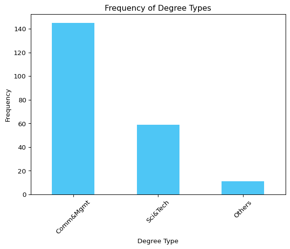
import matplotlib.pyplot as plt

# Plot the frequency of the original dataset
real_data["degree_type"].value_counts().plot(kind="bar", color="#03AFF1", alpha=0.7)
plt.title("Frequency of Degree Types")
plt.xlabel("Degree Type")
plt.ylabel("Frequency")
plt.xticks(rotation=45)
plt.show()

The bar chart shows the imbalanced distribution of the degree_type column, with some categories being significantly more frequent than others. This imbalance can lead to biased synthetic data generation if not addressed.

UniformEncoder

The UniformEncoder from the RDT library solves this problem by transforming categorical columns into a uniform numerical distribution. This ensures that the encoded values are evenly distributed, preserving the original data’s characteristics.

from rdt import HyperTransformer
from rdt.transformers import UniformEncoder


# Use HyperTransformer to detect and apply transformations
transformer = HyperTransformer()

transformer.set_config(
    {
        "sdtypes": {"degree_type": "categorical"},
        "transformers": {"degree_type": UniformEncoder()},
    }
)


# Transform the data
transformed_data = transformer.fit_transform(real_data)
transformed_data.head()

	degree_type
0	0.222982
1	0.228482
2	0.625732
3	0.073374
4	0.327050

The UniformEncoder maps each category to a unique numerical value between 0 and 1, ensuring uniform distribution.

Let’s compare the encoded values with the original categorical data:

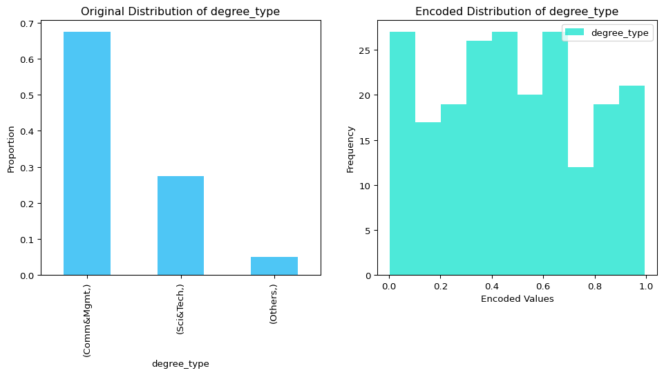
# Create a figure with two subplots
fig, (ax1, ax2) = plt.subplots(1, 2, figsize=(12, 5))

# Plot the original distribution on the first subplot
real_data.value_counts(normalize=True).plot(
    kind="bar", color="#03AFF1", alpha=0.7, label="Original Data", ax=ax1
)
ax1.set_title("Original Distribution of degree_type")
ax1.set_ylabel("Proportion")

# Plot the encoded distribution on the second subplot
transformed_data.plot(
    kind="hist", bins=10, color="#01E0C9", alpha=0.7, label="Encoded Data", ax=ax2
)
ax2.set_title("Encoded Distribution of degree_type")
ax2.set_ylabel("Frequency")
ax2.set_xlabel("Encoded Values")

plt.show()

The first plot shows the imbalanced distribution of the original categorical data, while the second plot demonstrates how the UniformEncoder transforms the data into a uniform numerical distribution.

Next, we can use the transformed data for synthetic data generation.

from sdv.single_table import GaussianCopulaSynthesizer

# Initialize and fit the synthesizer
synthesizer = GaussianCopulaSynthesizer(metadata)
synthesizer.fit(transformed_data)

# Generate synthetic data
synthetic_data = synthesizer.sample(num_rows=100)

# Reverse transform the synthetic data
reversed_data = transformer.reverse_transform(synthetic_data)

# Display the reversed column
reversed_data.head()

	degree_type
0	Others
1	Sci&Tech
2	Comm&Mgmt
3	Sci&Tech
4	Comm&Mgmt

The reverse_transform method converts the numerical values back to their original categorical form, making the synthetic data interpretable.

Finally, we can evaluate the quality of the synthetic data.

from sdv.evaluation.single_table import get_column_plot

# Visualize the distribution of the real and synthetic data
fig = get_column_plot(
    real_data=real_data,
    synthetic_data=reversed_data,
    metadata=metadata,
    column_name="degree_type",
)
fig.show()

This plot compares the distribution of the degree_type column in the real and synthetic datasets, demonstrating how well the UniformEncoder preserves the original data’s characteristics.