Building the Unique Combinations Constraint in the SDV

By default, a machine learning model (ML) may not always learn the deterministic rules in your dataset. We've previously explored how the SDV allows user to input their logic using constraints. With constraints, an SDV model produces logically correct data 100% of the time.

While an end user might expect the constraint to "just work," engineering this functionality requires some creative techniques. In this article, we'll describe the techniques we used to build the UniqueCombinations constraint. You can also follow along in our notebook.

!pip install sdv==0.13.1

import numpy as np
import warnings

warnings.filterwarnings('ignore')

What is a Unique Combinations Constraint?

Users frequently encounter logical constraints on the permutations -- mixing & matching -- that are allowed in synthetic data.

To illustrate this, let's use the world_v1 dataset from the SDV tabular dataset demos. This simple dataset describes the population of different cities around the world.

from sdv.demo import load_tabular_demo

data = load_tabular_demo('world_v1')
data = data.drop(['add_numerical'], axis=1) # not needed for this demo
data.head()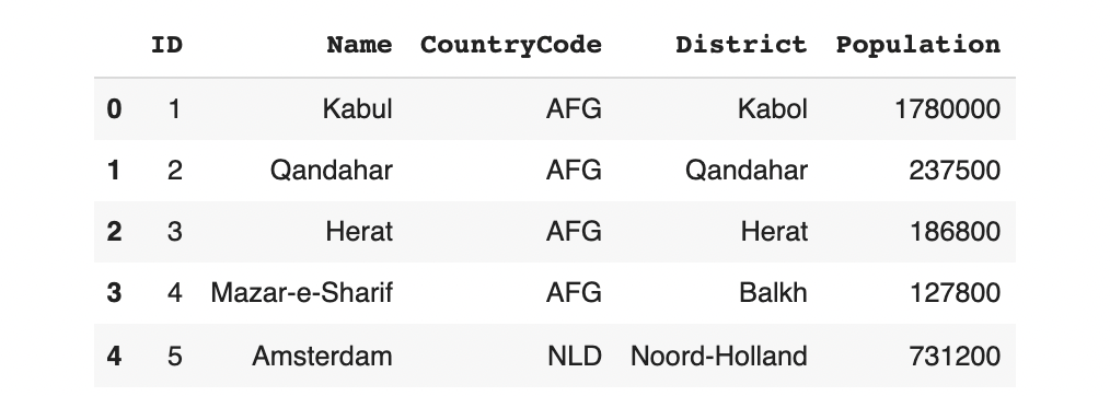

Relationship between Name, CountryCode and District

Looking at the data, we can observe that there is a special relationship between the Name of the city, its CountryCode and its geographical District: When generating synthetic data, the model should not blindly mix-and-match these values. Instead, it should reference the real data to verify whether the combination is valid. This is called a UniqueCombinations constraint.

For example, take a particular city, like Cambridge, which appears 3 times in our dataset.

data[data.Name == 'Cambridge']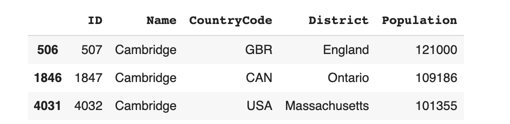

The constraint states that Cambridge should only ever appear with GBR (England), CAN (Ontario) or USA (Massachusetts). It is invalid if it appears in any other region -- for eg. Cambridge, France.

How does the SDV handle a Unique Combination out-of-the-box?

Let's try running the sdv as-is on the dataset to see what happens. We'll use the GaussianCopula model on our dataset.

from sdv.tabular import GaussianCopula

np.random.seed(0)

model = GaussianCopula(
  categorical_transformer='label_encoding' # optimize speed
) 
model.fit(data)

Now, let's generate some rows to inspect the synthetic data.

np.random.seed(12)
model.sample(5)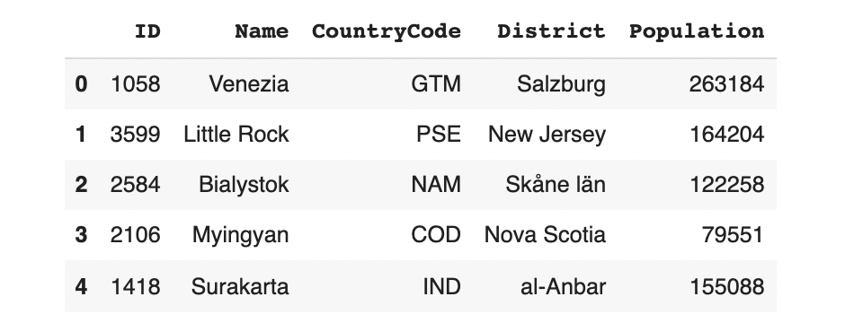

Although the sdv is generating known city names, countries and districts, their combinations don't make sense. We can also go back to our original example and generate only some rows for Cambridge.

np.random.seed(10)

conditions = {'Name': 'Cambridge'}
model.sample(5, conditions=conditions)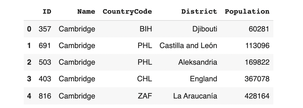

The result is a variety of Cambridges that aren't necessarily in USA, GBR, or CAN. These aren't valid cities!

What's going on? The SDV models include probabilities that some unseen combinations are possible. This is by design: Synthesizing new combinations -- that don't blatantly match the original data -- helps with privacy.

However in this particular case, we aren't worried about the privacy of a city belonging to a country or district. We actually do want the data to match. This is why we need to build a constraint.

Fixing the data using rejecting sampling

In our previous article, we described a solution called reject_sampling that works on any type of constraint and is very easy to build: We simply create the synthetic data as usual and then throw out (reject) any data that doesn't match.

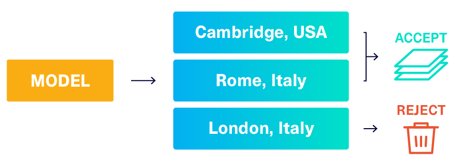
In theory, this can solve our UniqueCombinations constraint. In practice, this strategy is only efficient if the model can easily generate acceptable data. Let's calculate the chances of getting an acceptable combination (Name, CountryCode, District) from the model.

np.random.seed(0)

# Sample data from the model
# The sample may include combinations that aren't valid
n = 100000
new_data = model.sample(n)

# Calculate how many rows are valid
combo = ['Name', 'CountryCode', 'District']
merged = new_data.merge(data, left_on=combo, right_on=combo, how='left')
passed = merged[merged['ID_y'].notna()].shape[0]

# Print out our results
print("Valid rows: ", (passed/n)*100, "%")
print("Rejected rows: ", (1 - passed/n)*100, "%")

Valid rows:  0.038 %
Rejected rows:  99.96199999999999 %

With such a low probability of passing the constraint, this strategy can become intractable.

Fixing the data using transformations

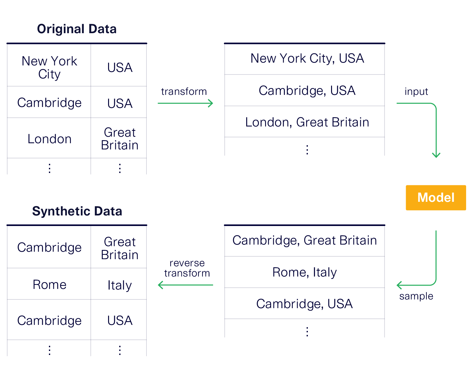
A more efficient strategy is for the ML model to learn the constraint directly, so it always produces acceptable data. We can do this by transforming the data in a clever way, forcing the model to learn the logic.

Our previous article described how to do this for a different constraint. Unfortunately, the exact same transformation won't work to solve our current UniqueCombinations constraint. The transform strategy requires a different, creative solution for each constraint. So we have to start from scratch.

Can you think of any other ways to enforce UniqueCombinations?

A solution: Concatenating the data

One solution is to concatenate the data. That is, rather than treating the city Name, CountryCode and District as separate items, we treat them as a single value. This will force the model to learn them as 1 single concept rather than as multiple columns that can be recombined.

Let's see this in action.

# create transformed data that concatenates the columns
data_transform = data.copy()

# Concatenate the data using a separator
data_transform['concatenated'] = data_transform['Name'] + '#' + data_transform['CountryCode'] + '#' + data_transform['District']

# We can drop the individual columns
data_transform.drop(labels=['Name', 'CountryCode', 'District'],
                    axis=1, inplace=True)

data_transform.head()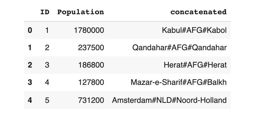

Now, we can train the model using the transformed (concatenated) data instead.

np.random.seed(35)

# create a new model that will learn from the transformed data
model_transform = GaussianCopula(categorical_transformer='label_encoding')
model_transform.fit(data_transform)

# this will produce transformed data
output = model_transform.sample()
output.head(5)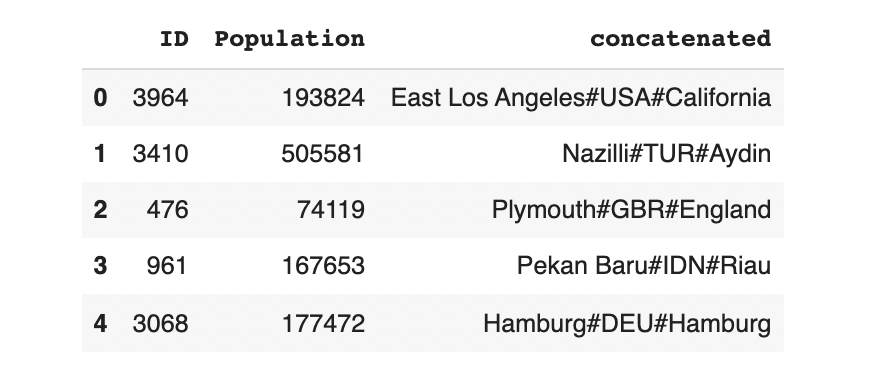

To get back realistic-looking data, we can convert the concatenated column back into Name, City and District.

import pandas as pd

# Split the conatenated column by the separator and save the reuslts
names = []
countrycodes = []
districts = []

for x in output['concatenated']:
  try:
    name, countrycode, district = x.split('#')
  except:
    name, countrycode, district = [np.nan]*3
  names.append(name)
  countrycodes.append(countrycode)
  districts.append(district)

# Add the individual columns back in
output['Name'] = pd.Series(names)
output['CountryCode'] = pd.Series(countrycodes)
output['District'] = pd.Series(districts)

# Drop the concatenated column
output.drop(labels=['concatenated'], axis=1, inplace=True)

As a result, the output now looks like our original data.

output.head()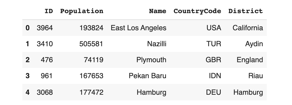

Most importantly, the Name, CountryCode and District columns now make sense!

Caveats of transforming the data

The transform strategy is an efficient and elegant approach to modeling. But there is a downside: The transform strategy might lose some mathematical properties.

To see why, consider the model's perspective:

• Cambridge#GBR#England is completely different from
• Cambridge#USA#Massachusetts is completely different from
• Boston#USA#Massachusetts

The problem is that two of these actually have something in common -- they are located in Massachusetts, USA. So the model will not be able to learn anything special about Massachusetts or USA as a whole.

As an example, let's see how well the model was able to learn populations of US-based cities.

import matplotlib.pyplot as plt

# Populations of real US cities
real_usa = data.loc[data['CountryCode'] == 'USA', 'Population']

# Populations of synthetic US cities
synth_usa = output.loc[output['CountryCode'] == 'USA', 'Population']

# Plot the distributions
plt.ylabel('US City Data')
plt.xlabel('Population')
_ = plt.boxplot([real_usa, synth_usa],
                showfliers=False,
                labels=['Real', 'Synthetic'],
                vert=False
)
plt.show()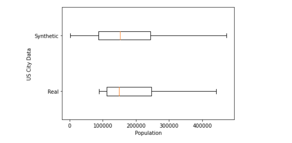

The real data shows less variation in city population than the synthetic data. The differences make sense because our model wasn't able to learn about the USA as one complete concept.

Can we fix this? It's challenging to fix this issue without degrading the mathematical correlations in some other way. If you have any ideas, we welcome you to join our discussion!

Inputting a UniqueCombination into the SDV

We built the constraint -- both the reject_sampling and transform approaches -- directly into the SDV library. If you have sdv installed, this is ready to use. Import the UniqueCombinations class from the constraints module.

from sdv.constraints import UniqueCombinations

# Create a Unique Combinations constraint
unique_city_country_district = UniqueCombinations(
  columns=['Name', 'CountryCode', 'District'],
  handling_strategy='transform' # you can change this 'reject_sampling' too
)

# Create a new model using the constraint
updated_model = GaussianCopula(
  constraints=[unique_city_country_district],
  categorical_transformer='label_encoding'
)

Now, you can train the model on your data and sample synthetic data.

np.random.seed(35)

updated_model.fit(data)
updated_model.sample(5)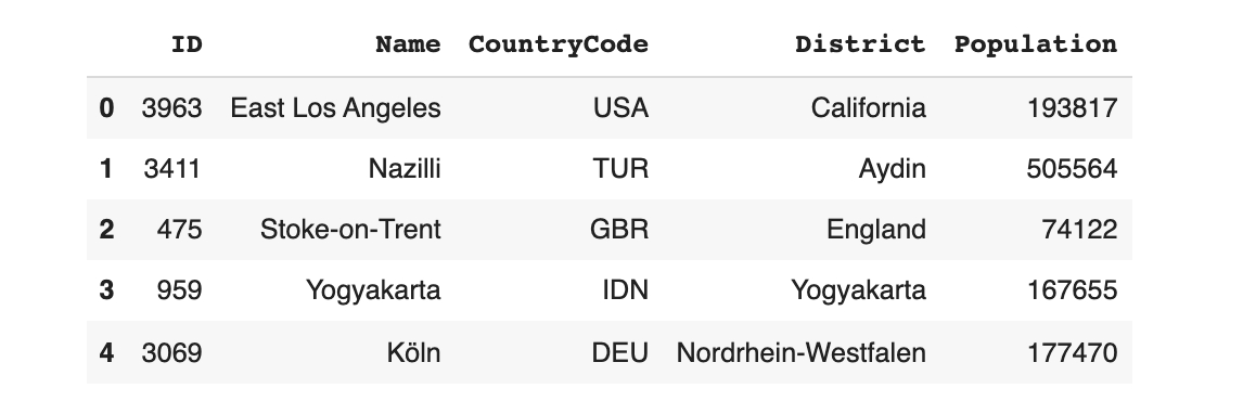

All of the synthetic data is guaranteed to follow the UniqueCombinations constraint.

Takeaways

1. We can identify a UniqueCombinations requirement by asking: Should it be possible to further mix-and-match the data?
2. We can enforce any logical constraint by using reject sampling, which throws out any invalid data. This is not efficient for UniqueCombinations.
3. An alternative approach is to transform the data, forcing the ML model to learn the constraint. For UniqueCombinations we transformed the data by concatenating it.
4. The logic for UniqueCombinations is already built into the SDV's constraints module, and is ready to use.

Further reading:

• Engineering Constraints Blog Article
• Handling Constraints User Guide
• Tabular Constraints API