Interpreting the Progress of CTGAN

This article was researched by Santiago Gomez Paz, a DataCebo intern. Santiago is a Sophomore at BYU and an aspiring entrepreneur who spent his summer learning and experimenting with CTGAN.

This article was edited on Feb 29, 2024 to match the updated API for SDV version 1.0+.

The SDV library offers many options for creating synthetic data tables. Some of the library's models use tried-and-true methods from classical statistics, while others use newer innovations like deep learning. One of the newest and most popular models is CTGAN, which uses a type of neural network called a Generative Adversarial Network (GAN).

Generative models are a popular choice for creating all kinds of synthetic data – for example, you may have heard of OpenAI's DALL-E or ChatGPT tools, which use trained models to create synthetic images and text respectively. A large driver behind their popularity is that they work well — they create synthetic data that closely resembles the real deal. But this high quality often comes at a cost.

Generative models can be resource-intensive. It can take a lot of time to properly train one, and it's not always clear whether the model is improving much during the training process.

In this article, we'll unpack this complexity by performing experiments on CTGAN. We'll cover:

• A high-level explanation of how GANs work
• How to measure and interpret the progress of CTGAN
• How to confirm this progress with more interpretable, user-centric metrics

You can replicate all the work in this post using this Colab notebook.

How do GANs work?

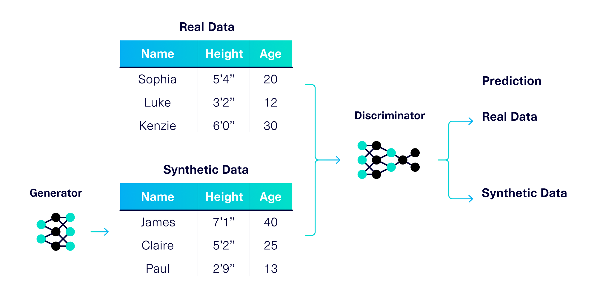
Before we begin, it's important to understand how GANs work. At a high level, a GAN is an algorithm that makes two neural networks compete against each other (thus the label “Adversarial”). These neural networks are known as the generator and the discriminator, and they each have competing goals:

• The discriminator's goal is to tell real data apart from synthetic data
• The generator's goal is to create synthetic data that fools the discriminator

The setup is illustrated below.

This setup allows us to measure – and improve – both neural networks over many iterations by telling them what they got wrong. Each of these iterations is called an epoch, and CTGAN tracks inaccuracies as loss values. The neural networks are trying to minimize their loss values for every epoch.

The CTGAN algorithm calculates loss values using a specific formula that can be found in this discussion. The intuition behind it is shown below.

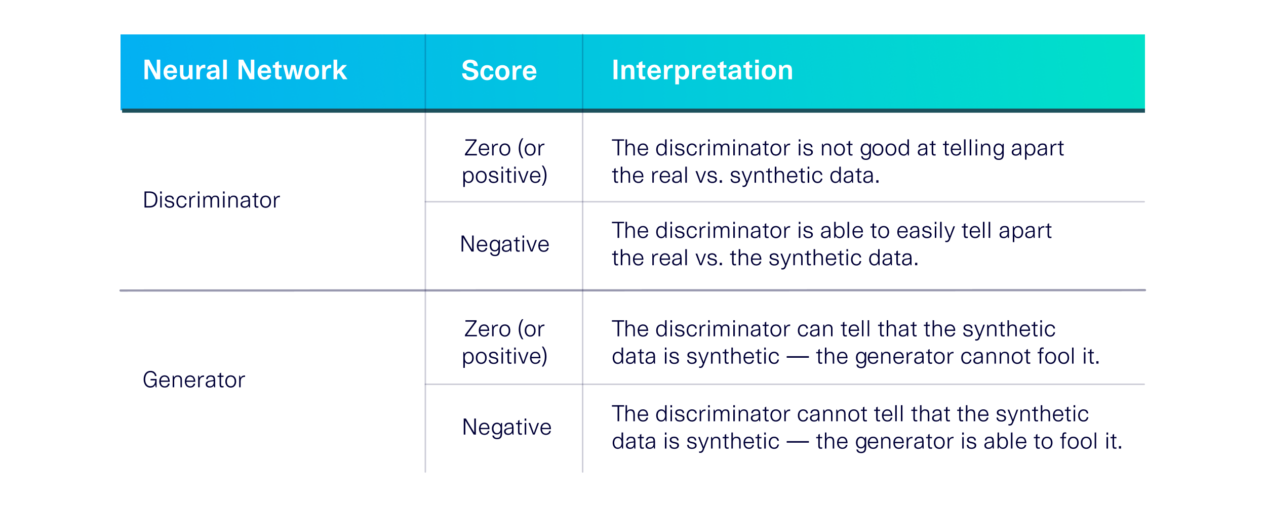
As shown by the table, lower loss values – even if they are negative – mean that the neural networks are doing well.

As the epochs progress, we expect both neural networks to improve at their respective goals – but each epoch is resource-intensive and takes time to run. A common request is to find a tradeoff between the improvement achieved and the resources used.

Measuring progress using CTGAN

The open source SDV library makes it easy to train a CTGAN model and inspect its progress. We'll train a CTGAN model using a publicly available SDV demo dataset named census_extended, which contains some fake census data.

from sdv.datasets import demo

# Return list of demo datasets
demos_df = get_available_demos(modality='single_table')

# Save dataset as a dataframe & metadata
data, metadata_obj = download_demo('single_table', 'adult')

data.head()

Here's what the dataset looks like:

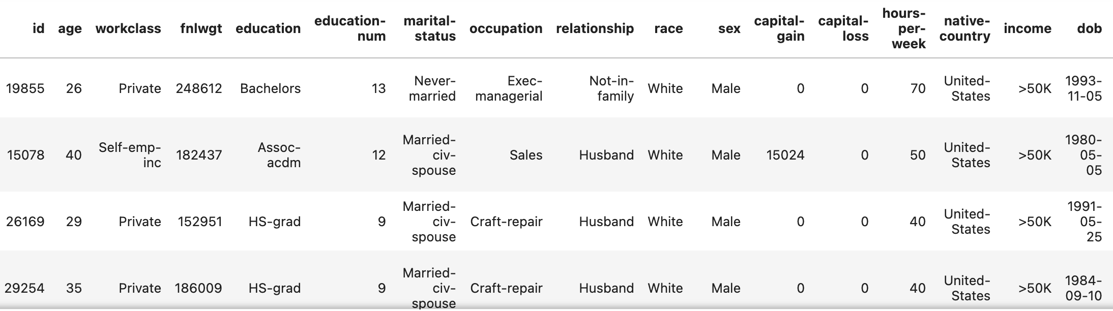
In addition to the dataset itself, we're given metadata about the dataset as a SingleTableMetadata object (which we assigned to metadata_obj). Next, we're ready to train a CTGAN model using the friendly CTGANSynthesizer class.

from sdv.single_table import CTGANSynthesizer

synthesizer = CTGANSynthesizer(metadata_obj, epochs=2000, verbose=True)
synthesizer.fit(data)

As part of the fitting process, CTGAN trains the neural networks for multiple epochs. After each epoch, it prints out the count, the generator loss (G) and the discriminator loss (D). Keep in mind that lower numbers are better – even if they are negative.

To see how the neural networks are improving, we plot the loss values for every epoch. The results from our experiment are shown in the graph below.

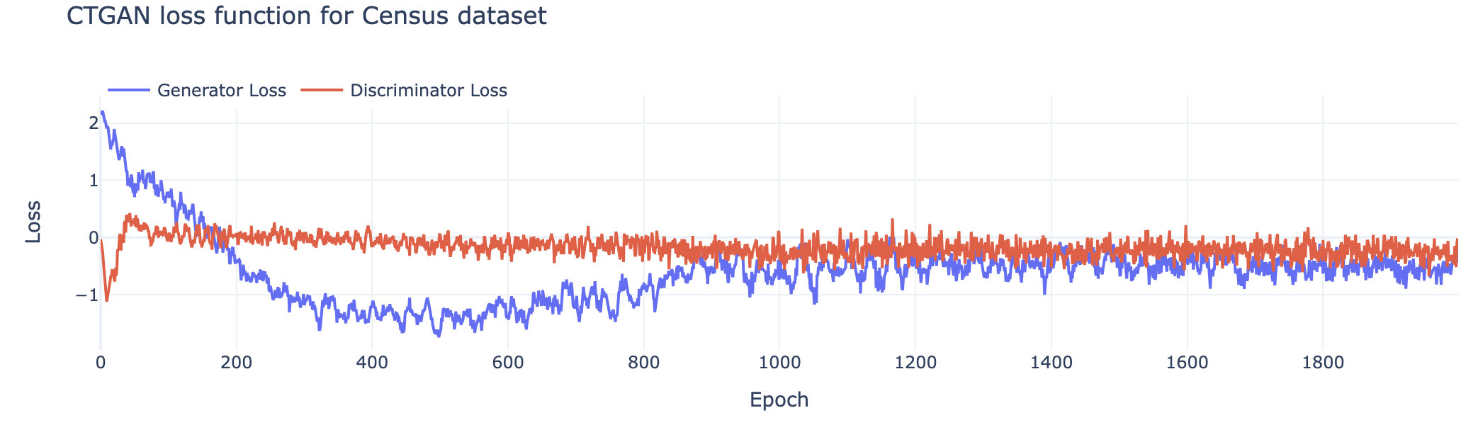
Based on the characteristics of this graph, it's possible to understand how the GAN is progressing.

Interpreting the loss values

The graph above may seem confusing at first glance: Why is the discriminator's loss value score oscillating at 0 if it is supposed to improve (minimize and become negative) over time? The key to interpreting the loss values is to remember that the neural networks are adversaries. As one improves, the other must also improve just to keep its score consistent. Here are three scenarios that we frequently see:

1. Generator loss is slightly positive while discriminator loss is 0. This means that the generator is producing poor quality synthetic data while the discriminator is blindly guessing what is real vs. synthetic. This is a common starting point, where neither neural network has optimized for its goal.
2. Generator loss is becoming negative while the discriminator loss remains at 0. This means that the generator is producing better and better synthetic data. The discriminator is improving too, but because the synthetic data quality has increased, it is still unable to clearly differentiate real vs. synthetic data.
3. Generator loss has stabilized at a negative value while the discriminator loss remains at 0. This means that the generator has optimized, creating synthetic data that looks so real, the discriminator cannot tell it apart.

Here are some other examples of loss charts from other datasets.

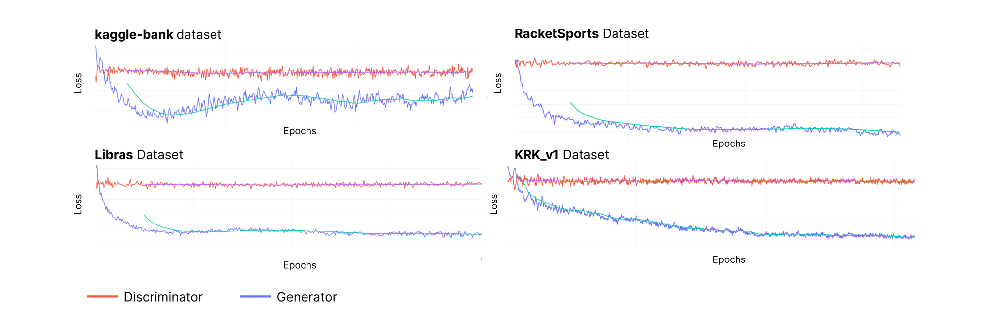
Of course, other patterns may be possible for different datasets. But if loss values are not stabilizing, watch out! This would indicate that the neural networks were not able to effectively learn patterns in the real data.

Metrics-Powered Analysis

Evaluating Single Columns

You may be wondering whether to trust the loss values. Do they indicate a meaningful difference in synthetic data quality? To answer this question, it's helpful to create synthetic data sets after training the model for different numbers of epochs, and assess the quality of the data sets.

synthetic_data = synthesizer.sample(num_rows=len(data))

It is important to select a few key metrics for a quantifiable quality measure. For our experiments, we chose 4 metrics from the open source SDMetrics library:

• KSComplement evaluates the shape of numerical columns
• TVComplement evaluates the shape of discrete columns
• CorrelationSimilarity evaluates pairwise correlations between columns
• CategoryCoverage evaluates whether the synthetic data covers all possible values

Each metric produces a score ranging from 0 (worst quality) to 1 (best quality). In the example below, we use the KSComplement metric on a numerical column in the dataset.

from sdmetrics.single_column import KSComplement

NUMERICAL_COLUMN_NAME='hours-per-week'

score = KSComplement.compute(
   data[NUMERICAL_COLUMN_NAME],
   synthetic_data[NUMERICAL_COLUMN_NAME])

Our results validate that the scores do, indeed, correlate with the loss value from the generator: The quality improves as the loss is minimized. Some of the metrics – such as CorrelationSimilarity and CategoricalCoverage – are high to begin with, so there is not much room to improve. But other metrics, like KSComplement, show significant improvement.

It's also possible to visualize the synthetic data that corresponds to a specific metric. For example, KSComplement compares the overall shape of a real and a synthetic data column, so we can visualize it using histograms.

from sdmetrics.reports import utils

utils.get_column_plot(
  data,
  synthetic_data,
  column_name=NUMERICAL_COLUMN_NAME,
  metadata=table_metadata)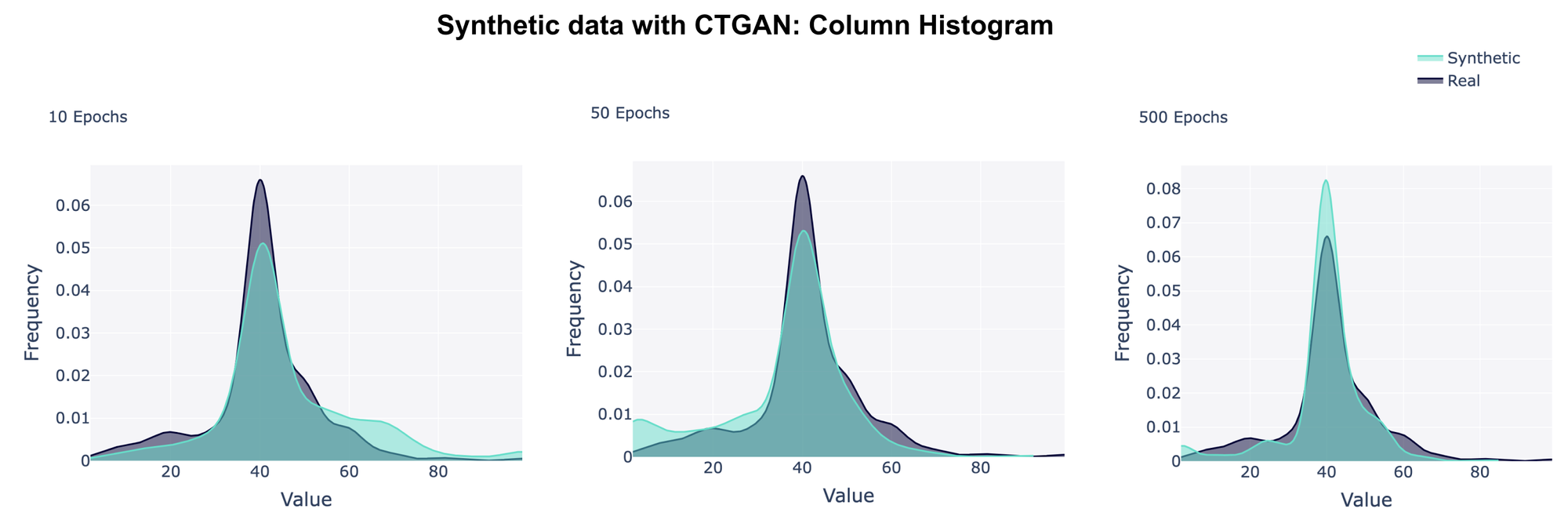

Overall, we can conclude that the generator and discriminator losses correspond to the quality metrics that we measured – which means we can trust the loss values, as well as the synthetic data that our CTGAN created!

Evaluating Multiple Columns

To make it even easier to understand model quality while you're iterating, we've created functions for automatically calculating these metrics across all columns. We can use the QualityReport class from sdmetrics to generate dataset-level reports. The easiest way to generate and interact with this quality report is through sdv.

from sdv.evaluation.single_table import evaluate_quality

quality_report = evaluate_quality(
    real_data=data,
    synthetic_data=synthetic_data,
    metadata=metadata)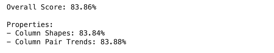

The quality report calculates:

• Column Shape score: average of all the quality scores for each column (pairing the appropriate metric with the column type). Greater than 80% is a great score.
• Column Pair Trends score: average pair-wise column correlation to help you understand how well the trend between pairs of columns were captured by the model. Greater than 80% is a great score.

You can dive into the specific column scores using:

fig = quality_report.get_visualization(property_name='Column Shapes')
fig.show()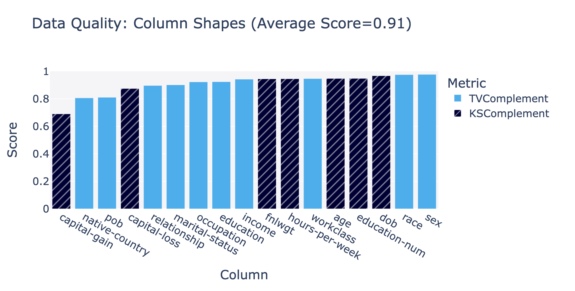

Conclusion

In this article, we explored the improvements that the CTGAN model makes as it iterates over many epochs. We started by interpreting the loss values that each of the neural networks – the generator and the discriminator – reports over time. This helped us reason about how they were progressing. But to fully trust the progress of our model, we then turned to the SDMetrics library, which provides metrics that are easier to interpret. Using this library, we could verify whether the reported loss values truly resulted in synthetic data quality improvements.

What do you think? If you've used CTGAN for synthetic data generation, we'd love to hear from you in the comments or in our Slack!